.png?width=200&height=52&name=Adikteev-H-White%20(1).png)
In our last article, we covered the various methodologies used to conduct an incrementality test for your app. But let’s say you’ve already run an incrementality test and gotten amazing results. How do you know if your results aren’t just a fluke? In this article, we’ll dive into how to determine the statistical significance of your incrementality test results.
Statistical significance Part I: What is it and why do we need it?
During the past months, methodology has been a key topic when looking at the different medical studies performed on drugs and vaccines in development to fight COVID-19. It should go without saying, but it’s essential that scientists and researchers first establish any treatment’s incremental benefit, statistical significance, and clinical importance. Simply put, they have to ensure that the incrementality test that they’ve run on a specific drug or treatment actually produced results that are accurate.
What is statistical significance?
Statistical significance measures the possibility that the difference between the control and test groups is not just due to chance. It’s a way to ensure that the results of an incremental test are correct and not just pure luck.
When looking at any incremental test result, statistical significance is as important as both the percentage of lift and the way of segmenting the subjects. Significance will tell you in the end if the percentage you’re looking at really means something.
How to determine statistical significance
We can summarize statistical significance as 2 key metrics for the given hypothesis we’re testing: p-value and confidence intervals.
- The p-value, or probability value, represents the probability of getting test results at least as extreme as the results obtained during the test, assuming that the null hypothesis is correct. We’ll get into the null hypothesis later on.
- The confidence interval estimates the range within which the real results would fall if the trial is conducted many times. A 95% confidence interval indicates that in 95% of the trials, the results would fall within the same range.
In other words, when running an incrementality test we must:
- Randomly split the audience between 2 groups: control & test as explained in our previous blog post. The test group will receive the treatment, or see the ads, and the control group will not.
- Make the hypothesis that the difference observed between control and test groups is due only to each group’s variability.
- Ensure that the two groups are homogeneous. We must calculate a probability that only variability explains the observed difference between each group: the p-value. If there is less than 5% of chance that the observed differences are due to variability alone (p-value <5%), the test is statistically significant. On the contrary, if there is a greater than 5% chance (p-value >5%), the difference might be due only to chance. A good way around this is to increase the size of the groups, or lengthen the time frame.
Here’s an example:
For an app, we want to run two distinct in-app re-engagement campaigns on two segments. Let’s call them segment A and segment B. We want to run an incrementality test on those campaigns to assess if we’ve generated incremental revenue.
As explained in our previous blog post, both audience segments will be split randomly into two groups: control & test.

After 30 days of the campaign, we compute the results.

Looking at those results, it seems we can conclude that both campaigns generated incremental average revenue per user (ARPU). But as we stated at the end of our last article, this isn’t not enough to draw any conclusions. We must make sure those results are not due to chance.
To do so, let’s take a closer look now at the statistical significance of those results.

As explained previously, we can see that segment A has a p-value of 0.02 (<5%), which means that there is less than 2% of chance that the results are due to variability alone. We can safely conclude here that the results are significant and the campaign really generated an uplift of +16.4%
Now let’s look at segment B. Despite very good lift percentage results, the p-value reached 0.13 (>5%). It means that it’s not significant enough to conclude anything. If we want to accurately test segment B, we need to increase its size to have a wider audience or extend the timeframe of the analysis.
Statistical significance Part II: How to read and understand the results
Now that the concept of statistical significance is clearer, we’ll dig into the different statistical tests Data Science & Analytical teams usually run to calculate the p-value.
We’ll start by outlining the questions we must answer before running a test. Then, we’ll introduce two different types of statistical tests: parametric and nonparametric. Finally, we’ll explain how they work and how we use them at Adikteev.
Statistical significance tests: The basics
There’s a ton of information available about statistical significance tests. For an in-depth understanding of the topic we recommend reading Erich L. Lehmann and Joseph P. Romano’s Testing Statistical Hypotheses [7]. If you’re interested how the field has developed over time, have a look at Ronald Fisher’s “The Design of Experiments” [6]. For this blog post, we’re going to focus on the practical side with some quick guidelines.
Before carrying out a statistical significance test it’s essential to define these six points ahead of time:
- The metrics you want to consider during the experiment. These can be categorical, binary, continuous, strictly positive, etc.
- The null and alternative hypotheses you would like for the test
- An appropriate statistical test with its test statistic
- The confidence level, defined as a type 1 error. This is known as the rejection of a true null hypothesis, which we’ll outline later.
- The treatment and control groups created without any potential bias, usually by randomization as we mentioned before.
- Estimated group sizes necessary to draw conclusions at the end of the experiment.
Statistical guarantees behind most of the methods of experimental design and statistical hypothesis testing come from the fundamental results of statistics and probability theory, in particular the law of large numbers and the central limit theorem. Note that more advanced techniques allowing sequential testing have emerged from another branch of probability and statistics called Bayesian probability theory, which we’ll briefly touch on at the end of this post.
What to consider when building a statistical significance test
Regardless of the type of statistical significance test you’re running, there are some general considerations to keep in mind.
As mentioned earlier, it’s essential to define a hypothesis ahead of time. The statistical significance test will validate or disprove an assumption we make about parameters of a statistical model. For instance we can define the probability values, p1 and p2, as the likelihood that two sub-groups of app users will make a conversion. We are interested in testing the hypothesis “p1 > p2”, or users in group 2 are more likely to make a conversion than users in group 1.
Sample size and confidence level
This is where sample size and confidence level come into play:
Sample size: Without a decent number of observations (i.e. sample size) conclusions might be unreliable. “My toothpaste makes teeth whiter. This is proven by an independent scientific study on 5 different individuals.”
Confidence level: We’ve covered confidence intervals, but If we want to say yes or no about our hypothesis, we need to agree in advance on a confidence level (say 95%) above which we can conclude. The confidence level is the percentage of confidence intervals that contain the population mean.
A confidence level of 95% means that if we were to conduct the experiment an infinite number of times, 95% of the time we would get the right conclusion. We’ll come back to that last point in more detail later on.
FYI: we should always decide on a confidence level before running the experiment or avoid looking at the data and test results if we haven’t yet decided on one. Otherwise it might be tempting to choose the “right” level to “pass” the test and reject or validate our hypothesis every time.
Type 1 & 2 errors, and the “null hypothesis”
But there’s a twist with hypothesis testing: when performing statistical significance tests we actually need two hypotheses. We might only be interested in finding out if users from group 2 are more likely to make conversions than users from group 1. But by doing this we implicitly define another alternative hypothesis: users from group 2 are no better than users from group 1. This is called H0 or “null hypothesis.” In order to construct a statistical test we actually need two hypotheses: H1 versus H0. Our goal is to reject H0 in order to conclude.
But there’s always a chance that we’ve gone wrong somewhere. These are probabilities, and we can’t be 100% sure. For instance we might reject H0 while it was true or might not have rejected it while we should have. We can sum up these situations in a two-by-two table:

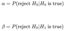
According to the table, if we get a true negative or true positive, we were right. Otherwise we were incorrect. So what does it mean to be 95% sure? Typically, a 95% confidence level means that the probability of a type 1 error occurring, given the null hypothesis is actually true, is 5% (100% - 95% confidence).
Much like with deciding on a confidence level after running an experiment, it may be tempting to consider designing a test that always chooses not to reject H0. This would lead to 100% confidence. However, a test designed this way would be useless. We want a test with a decent confidence level, but one that doesn’t take 1 billion samples to reject H0. We call this the power of a statistical test (1 - β for math people, and ɑ is the significance). The power is the probability that H0 will be rejected because H1 is true.
So in a nutshell:
A good test gives a high ![]() given
given ![]() (
( ![]() =0.05 usually)
=0.05 usually)
An optimal test maximizes ![]() given
given ![]() (
( ![]() =0.05 usually)
=0.05 usually)
This method does come with some limitations. You can find most of them listed in [4] section 3.6. Maybe the most well-known limitation is named by the authors as “primacy and newness effects.” To give an example from our work at Adikteev, introducing a new app feature that we would like to test in parallel with an existing test may produce a positive or negative temporary bias. The novelty of this feature and short-term user interest might cloud the test we’re trying to run on a campaign.
Parametric tests
In the previous section we’ve described how to play with test hypotheses and to interpret test results. But we still need to define what makes up the core of a statistical significance test. How do we know if we reject the null hypothesis or not? This is where parametric and non-parametric tests differ. Let’s first look at parametric ones.
A parametric statistical significance test assumes data coming from a population follows a given distribution (e.g., normal, Bernoulli), or by parameters. Our null hypothesis will involve a quantity derived from those parameters.
If we have enough samples, a classic trick is to use the central limit theorem (CLT) to approximate distributions with normal ones. Using math, we derive the distribution of the quantity of interest (let’s say the mean) under the null hypothesis. We then compare this distribution with the estimation we get from our data to see if it matches the hypothesis. For instance we might use a quantile that matches the desired confidence level. We’ll then agree that if the empirical value is above this quantile, the value is too suspicious and we reject the null hypothesis.
Parametric tests through a practical example: the famous t-test
For example, we would like to know if app users in France spend more time in the app than their German counterparts on average. In this example the data is not paired and the two samples can be of different sizes. We’ll use the following sample sizes:
 Number of users in Germany vs. France
Just imagine we now have two big .csv or excel files containing 150k or 100k numbers that represent the amount of time in seconds each user spent in the app in a given month, week or day.
Active users can’t spend less than 1 second using the app, which means our variable of interest is positive. In this case, it’s useful to apply a logarithmic transformation for data to be closer to a Gaussian, or Normal distribution.
The test we use at Adikteev is called Student test, or 2-sample t-test (Snedecor and Cochran, 1989). This is one of the most well-known statistical tests, famous for giving undergrads nightmares. The basic idea is simple: we want to assess whether the means of the two distributions are equal.
Let’s say that ![]() are the German log-times and
are the German log-times and ![]() are the French ones. The true, and thus unknown, means are 1 and 2. The formal hypotheses are:
are the French ones. The true, and thus unknown, means are 1 and 2. The formal hypotheses are:
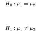
One can derive the test statistic which is:
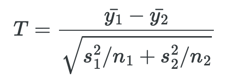
where ![]() and
and ![]() are the empirical means of both samples,
are the empirical means of both samples, ![]() and
and ![]() the empirical variances.
the empirical variances.
We reject the null hypothesis if ![]() where
where ![]() is the confidence level (e.g. 0.05) and v is called “degrees of freedom” and
is the confidence level (e.g. 0.05) and v is called “degrees of freedom” and ![]() is the 1−
is the 1−![]() quantile of the t distribution (aka student distribution) with vdegrees of freedom. We won’t go into the details of how
quantile of the t distribution (aka student distribution) with vdegrees of freedom. We won’t go into the details of how ![]() is computed. But a special case is worth noticing nonetheless: if the two empirical sample variances are equal then we have
is computed. But a special case is worth noticing nonetheless: if the two empirical sample variances are equal then we have ![]() . This means that the more data we have, the more Gaussian, or normal the t-distribution will look. The “- 2” actually accounts for computing the two empirical means
. This means that the more data we have, the more Gaussian, or normal the t-distribution will look. The “- 2” actually accounts for computing the two empirical means ![]() and
and ![]() . Check out [5] for further reading.
. Check out [5] for further reading.
Here’s an example of the test with simulated data in Python:


Because of the t-statistic value of 4.60 we can safely reject H0 and conclude that the difference is significant. Of course, we knew that from the beginning since we did simulate the data with different means. But in a real-life setting we would have to conclude from the t-statistic only.
Nonparametric tests:
Sometimes, parametric assumptions cannot be done when sample size is too small to apply asymptotic results. In this case, we use nonparametric tests instead. Nonparametric methods do not rely on data following a given parametric family of probability distributions. Because of this, they’re better when you’re facing skewed distributions. They’re also more robust in the presence of outliers, and more relevant when you are more interested in the median rather than in the mean. This is often the case at Adikteev when we are dealing with purchase amounts or number of conversions.
There are many nonparametric tests but for our uplift significance problem with large samples the Wilcoxon-Mann-Whitney test and Pearson’s chi-squared test are the most useful.
For significance tests involving purchase amounts or number of conversions, we use the Wilcoxon-Mann-Whitney test. There are a number of reasons for this but one is its ability to consider continuous data. The most common version of the test assumes that the distributions of both groups are identical. It formulates the alternative hypothesis as the distribution of one group being stochastically larger than the other. For those who are curious about the test statistic in more detail, it is derived after merging both samples and is calculated as a function of the sum of the ranks of each sample. More can be found in [3].
Bayesian A/B Test:
A test we don’t typically use when determining statistical significance but that deserves a mention is the Bayesian A/B test. This test is more flexible, less data is needed, and the response is not binary. It can also test multiple hypotheses at the same time, allows sequential testing, and there’s no need to wait for the predetermined time period to conclude.
Bayesian reasoning and testing is a vast area of study. The core idea compared to frequentist tests, or tests that only use data from the current experiment, is that we end up with a probability distribution of parameters that represent the hypothesis we want to test. In the case of a Bayesian test, we aren’t required to decide on a confidence level, although we can. We can use knowledge deduced about the problem from previous experiments or other sources using a prior distribution.
To sum up
As we mentioned at the beginning of this blog post, statistical significance testing is a vast topic. Here we’ve only scratched the surface to give you an idea of how we ensure our incrementality test results are accurate. However, there is a catch with incrementality measurement. Many marketers are in the habit of using return on ad spend (ROAS) as a main KPI, but measuring both ROAS and incrementality at the same time can actually hurt your campaign results. Stay tuned for our third and final article in this series to learn more about the difference between measuring ROAS and incrementality, and if there's a way to reconcile the two.
Subscribe to our newsletter so you don't miss it!


[1] Gelman, Andrew, et al. Bayesian data analysis. CRC press, 2013.
[2] Hastie, Trevor, Robert Tibshirani, and Jerome Friedman. The elements of statistical learning: data mining, inference, and prediction. Springer Science & Business Media, 2009.
[3] Wasserman, Larry. All of statistics: a concise course in statistical inference. Springer Science & Business Media, 2013.
[4] Kohavi, Ron, et al. "Controlled experiments on the web: survey and practical guide." Data mining and knowledge discovery 18.1 (2009): 140-181.
[5] Snedecor, George W., and William G. Cochran. "Statistical Methods, eight edition." Iowa state University press, Ames, Iowa (1989).
[6] Fisher, R. A. “The Design of Experiments” Oliver & Boyd (1935)
[7] Lehmann, E. L., & Romano, J. P. Testing statistical hypotheses. Springer Science & Business Media. (2006).